Regularization

Now you know about linear regression and logistic regression techniques. They work well for many problems but if you apply these techniques to certain applications, they can run into a problem of over-fitting which can degrade their performance. So what is over-fitting?
Suppose we have a data of housing prices varying as shown below by cross-marks, and we want to generate a model/function to estimate the varying curve,

Suppose we have 3 possible hypothesis,

Now we have to choose the best model out of these three (model selection). As we know that the aim of machine learning is to replicate the training data and prediction for new cases. Our model should be able to predict the right output for new cases. This is called generalization.

For best generalization, we should we should match the complexity of our hypothesis with the complexity of the function underlying the data. If the complexity of hypothesis is less complex than the function, we have under-fitting and if it is more complex, we have over-fitting.

So if we’ll have following scenario if we chose above hypothesis,

In first case, our hypothesis is less complex where as in third case it’s more complex, but in the second case, it is just right.
So if we have too many features, the hypothesis may fit the training set well but fail to generalize to new examples.

So how do we tackle this problem?

Options:

1. Reduce the number of features (later).
2. Regularization

Regularization:

In regularization, we reduce the magnitude of θ parameters. It works really well is we have lots of features and each of which contributes to value of y a bit. In our squared error function we add following term,

This term forces our coefficients values to a near zero region. And one thing to notice here is that we don’t minimize θ0, We only minimize θ1, θ2, …., θm.

Now how does this term effect our previously learned techniques? Let’s have a look.

Linear Regression

Our cost function becomes,

We just need to choose appropriate λ value. If we choose it very large, our result may suffer from under-fitting. Our gradient descent will be modified as,

On taking theta common outside, we get

Here 1 – αλ /m  < 1 always, so θj will be multiplied by a value less than 1. So it is minimizing.

Normal Equations

In normal equations case, our θ was

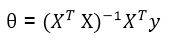
Here our equation changes to

I think you understood. Only first diagonal except first element are all ones and rest are zeros. It’s a matrix of (m+1) x (m+1).

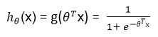
Logistic Regression

Its same as linear regression except the h(x) value will be sigmoid function here

grad = zeros(size(theta));
h = sigmoid(X*theta);
theta_reg = [0;theta(2:size(theta))];
J = (1/m)*( -y'*log(h) - (1-y)'*log(1-h) )+ ( lambda/(2*m) ) * theta_reg'*theta_reg;
grad=(1/m)*(X'*(h-y)+lambda*theta_reg);